Quantum jumps
The term “quantum jumps” refers to the apparently sudden transition of a quantum system from one state to another. For example, an electron bound to an atom can spontaneously jump to a lower energy, emitting a photon. Or an unstable atomic nucleus can spontaneously break apart, resulting in a state with part of the nucleus rapidly flying away.
The mystery of quantum jumps was one of the motivating forces for the development of quantum mechanics in the early 20th century. Bohr’s picture of the atom envisioned electrons orbiting the nucleus like planets orbiting the sun. From classical physics, one would expect these orbiting electrons to continuously emit light of increasing frequency, while spiralling in towards the nucleus. Instead, it was observed that atoms can only emit very specific frequencies. This was explained by the new quantum theory with the idea that the electron stays put in a state with a particular energy, then at some point, spontaneously jumps to a different state with lower energy. This jump occurs at a random time, apparently instantaneously.
The only problem with this explanation was that there wasn’t anything in quantum theory to really explain how this worked. The standard quantum theory developed in the first half of the 20th century has two parts. First, the Schrödinger equation tells us how a quantum wave function evolves continuously in time – there doesn’t seem to be any possibility of jumps here. The other part says that when a “measurement” is performed on a quantum system, the wave function spontaneously “collapses.” This does seem to offer the possibility of a sudden jump. The core of the problem, however, is that what constitutes a measurement is not well defined. Trying to apply this idea to pin down precisely how and when quantum jumps occur ends up getting us tied into all kinds of knots.
Ultimately, the mystery was finally solved in the 1990s (see “There are no Quantum Jumps, nor are there Particles!,” Dieter Zeh, Physics Letters A172, 189 (1993)). The solution rests only on the continuous evolution of the Schrödinger equation, discarding the postulate about measurements, as we have done throughout Catland. Also like what we have seen in Catland, the solution relies on interaction of the system with its environment, and subsequent entanglement and well-separated “worlds.” We will illustrate the argument here using the type of examples developed throughout Catland.
Our example here will be loosely based on the process of nuclear decay. The same idea should also apply to emission of photons, as we’ll discuss below.
Quantum jumps in nuclear decay are familiar to anyone who has used a Geiger counter. When brought near radioactive materials, a Geiger counter produces an audible click whenever it detects the emission of a particle from a nuclear decay. The result is a series of randomly timed clicks becoming more dense or sparse as the level of radioactivity increases or decreases. This leads to a picture where each radioactive nucleus, in any given short time interval, has some fixed probability of decaying. That is, the nucleus just sits there for some time, then at a randomly chosen moment splits apart. The details vary as to the specifics of what happens when the nucleus splits apart, but generally some particle or particles wind up getting emitted with a high energy. In perhaps the simplest case, a chunk of the nucleus (two protons and two neutrons bound together as an “alpha particle”) splits off and goes flying.
The typical time for a nucleus to decay (characterized by the half-life) varies dramatically – some isotopes are almost completely unstable, and others almost completely stable. But for many common radioactive materials, the half-lives are measured in years. For example, tritium, an isotope of hydrogen, has a half-life of 12.33 years. For this reason, materials incorporating tritium can be used to make glowing wristwatch dials. (If the half-life were very fast, like seconds or nanoseconds, the material would have decayed before it could even be applied in the watch factory. If the half-life were very slow, like billions of years, it wouldn’t be radioactive enough to visibly glow.) This means that if you have an atom of tritium and wait 12.33 years, there is a 50% chance it will have decayed by then. If it has not decayed by then, there is a 50% chance it will decay in the next 12.33 years.
Another example of a radioactive material is uranium. The most abundant naturally occurring isotope of uranium is U-238. Unlike tritium, this one decays via emission of an alpha particle (the case we will be picturing below). The half-life of U-238 is 4.5 billion years. This rather long decay time makes U-238 useful for determining the age of rocks via “radiometric dating.” If an atom of U-238 was incorporated into a rock that solidified when the earth was just formed about 4.4 billion years ago, there is now just about about a 50% chance that it will be found to have decayed, having emitted an alpha particle to become thorium-236 (which itself will decay further to other atoms). By looking at the ratio of U-238 atoms to its decay products, the age of the rock can be determined.
The example below will paint a rather different picture of the nuclear decay process. Instead of a sudden, randomly-timed decay, the wave function of the alpha particle will be continuously “leaking” out. The leaking might be extremely slow, like over billions of years in the case of U-238. Imagine a puddle of water slowly seeping out across the floor, from a water tank with a slow leak. It is the process of detecting the alpha particle that results in the appearance of fast jumps. These jumps will not be instantaneous, but instead set by the rate of some other interaction which may be much faster than the nuclear decay. So why does it look like a localized particle is emitted at a random, distinct time? (And for that matter, in a distinct direction?) This is the effect of interactions with other particles in the environment, leading to entanglement, decoherence, and our perception of just one of many “worlds”.
Nuclear decay toy model
As throughout Catland, we will simulate the wave function of one or several particles moving in one dimension. One particle will represent the alpha particle. We will impose an external potential meant to mimic the initial binding of the alpha particle to the rest of the nucleus. This potential is shown by the dashed red line in Fig J.1. The nucleus would be located in the region from about \(x=-24\) to \(-20\). This potential has barriers on either side of the nucleus to trap the alpha particle. (In reality, these barriers represent the binding due to the strong nuclear force.) The barrier on the right, however, is fairly narrow and with a finite height. As we will see, this means that the wave function won’t be completely trapped by that barrier. (The barrier on the left is much higher and wider so the alpha particle will be much more effectively trapped on that side. In reality, we would have symmetric barriers on all sides, and the wave function would leak in all directions. But this setup allows us to just focus on one side at a time.) Also, we see that bottom of the potential in the nucleus is greater than the potential outside. Therefore, any part of the wave function that leaks out will find itself with greater kinetic energy, due to the lower potential energy outside. In the case of actual nuclear decay, this occurs due to the repulsion of the positively charged alpha particle and the rest of the nucleus.
We will start the alpha particle with a so-called “metastable” wave function. This is a wave function that would be stable if the barrier on the right had an infinite width. The evolution of this wave function is shown in blue in the video in Fig J.1. The top panel shows the real and imaginary parts of the wave function, which shows a single bump within the well, just oscillating between the real and imaginary parts. The amplitude squared in the bottom panel just appears to be sitting there, doing nothing.
All-in-all the wave function in Fig J.1 looks pretty stable. But if we zoom in, we can see that it is metastable. The exact same wave function is shown in Fig J.2, with the vertical axis zoomed in. Now we can see the leakage of the alpha particle’s wave function out of the nucleus.
As the wave function begins to leak out, there is a period of initial rise, followed by some oscillations. After that, the leakage appears to be leveling off to a constant rate. If we were to continue the simulation, we would expect to see that leakage steadily continue for a very long time.
It is a mathematical fact that the area under the curve of amplitude squared remains constant over time as the wave function evolves. That makes the analogy with a leaky water tank particularly apt. As the water leaks out, we expect the water level in the tank to slowly decrease. The same should happen with the amplitude of the wave function still bound to the nucleus. In the time covered by the simulation in Fig J.1, this decrease is not yet visible. The rate of leakage is too slow (compare the scale of the vertical axes in Fig J.1 and Fig J.2). But if we waited long enough, we would see the amplitude squared of the bound portion reduce by half – this time would be the half-life.
As the amplitude of the bound part of the wave function decreases, we would also see the rate of leakage decrease. This is also not unlike how we might expect the water leakage to slow as the water level, and hence the water pressure, goes down. In other words, the amplitude of the leaking part of the wave function is proportional to the amplitude of the bound part. After one half-life, when the amplitude-squared still bound to the nucleus has reduced by one half, the amplitude-squared leaking out will also be reduced by one half. Eventually, after many half-lives, the amplitude remaining bound will become very small (though technically never zero), with a correspondingly small amount still leaking out.
Detecting nuclear decay
Now that we have seen how the alpha particle’s wave function slowly leaks out of the nucleus, we would like to detect it. Following the approach of Catland, we will first perform a “micromeasurement.” That is, a second microscopic system (a “detector”) will interact with the alpha particle, and that interaction will cause the detector’s state to evolve in some way that reveals information about the alpha particle. Following the micromeasurement, other particles will interact with the detector particle to amplify the information up to the macroscopic scale where we can perceive it (for example, ultimately producing an audible click.)
As in some previous sections of Catland, our detector will be modeled as a point-like two-state quantum system. The detector will interact with the alpha particle over some reasonably short range. In this case, the dependence of the interaction with distance will be given by a Gaussian function with a width of about 0.5 along the \(x\) axis. The result of this interaction is that, when the wave function has some amplitude close to the detector, the detector begins to rotate from one state to the other. In this case, the finite range of the interaction is such that the incoming particle will not reflect substantially due to the interaction as we saw for a much shorter range interaction in the Complementary observables section.
We could imagine the detector to be an electron bound to an atom. The electron will initially be in its lowest energy orbital – the ground state – which we will denote \(|g\rangle\). As the alpha particle wave function passes by, the amplitude in the \(|g\rangle\) state begins to transfer to an excited state, denoted \(|e\rangle\). Though the typical case would be that the excited state has a higher energy than the ground state, here we will take the two states to have the same energy. (It doesn’t change much if they have different energies, particularly if the energy difference is small compared to the kinetic energy of the incoming particle.)
First, we will look at how our detector responds to the passage of a generic wave packet. This is simulated in Figure J.3. The wave packet is initially at the left, and the detector is in the ground state. This is shown by the fact that the wave function appears in the top panel, correlated with the detector state \(|g\rangle\). As the packet moves past the detector, amplitude is transferred to the lower panel, which shows the part of wave function correlated with detector state \(|e\rangle\). After the wave packet has passed by, there are now two parts to the wave function: in the top panel, the detector remains in \(|g\rangle\) corresponding to an unsuccessful detection of the particle, and in the bottom panel, the detector is now in \(|e\rangle\) corresponding to a detection of the particle. (If we wanted to, we could tune the interaction so as to detect the packet with near-complete success, but it is more realistic to have only a partial chance of success with each interaction.)
Now applying the same detector to measure our nuclear decay, Fig. J.4 shows the simulated wave function where the alpha particle is now interacting with the detector, indicated by the dashed line. Now we are just showing the amplitude squared of the wave function, for simplicity. The action of the detector is similar as in the case of the simple wave packet. Once the alpha particle’s wave function has passed the detector, there is now some amplitude correlated with \(|e\rangle\), and a correspondingly reduced amplitude correlated with \(|g\rangle\).
There are a few subtleties to note in the interaction of the leaking alpha particle wave function with the detector in Fig. J.4. For one thing, the wave functions correlated with \(|g\rangle\) and \(|e\rangle\) are not the same. This also happened with the wave packet example in Fig. J.3 while the packet was partway through the detector, but it goes by pretty quickly. Here, the whole alpha particle wave function will take a long time (perhaps billions of years) to completely pass by the detector, so we will remain in this entangled state for a long time.
A second thing to note is that the part of the wave function that has passed the detector has already finished transferring amplitude to the \(|e\rangle\) component. One might think that because only a tiny fraction of the wave function has interacted with the detector, the detector would have barely been affected. In a sense, that is true. But to be accurate, each point of the wave function after the detector is correlated with the detector maximally activated. Each point of the wave function before the detector is correlated with the detector not activated at all.
A final comment about Fig. J.4 is that if we only look at the red wave function correlated with the detector being activated, there is no amplitude bound to the nucleus. This is a bit of foreshadowing. For now, there is no reason to only look at the red part. In fact, we could just as well split up the wave function into components in a different way, say into ones correlated with \(|g\rangle+|e\rangle\) and \(|g\rangle-|e\rangle\), which would both have equal amplitude bound to the nucleus. But for now, just imagining that we do want to consider the red and blue curves separately, the red curve corresponds to the detector being activated correlated with the complete decay of the nucleus.
Amplification and decoherence
If a single U-238 atom and a single detector atom were the only things in the universe, the slow decay and activation of the detector shown in Fig. J.4 would continue to play out over billions of years. Because the alpha particle is emitted at a significant fraction of the speed of light, the leaking wave function would spread out over a distance of a billion light-years or so.
Of course, these are not the only things in the universe. In fact, there are a great many things that we might expect to happen to either the alpha particle or the detector atom on vastly faster time scales. For example, a photon or air molecule may interact with the detector atom. These interactions might be intentional, leading to amplification and measurement, or accidental, leading to entanglement with the environment and decoherence.
We will consider a toy model of a particle in the environment interacting with the detector. We will refer to such a particle as a “probe particle.” The probe particles will initially be described by a single wave packet approaching the detector. The probe particle will interact with the detector in a simple way: if the detector is in the ground state \(|g\rangle\), the probe particle does not interact at all and passes by unaffected; if the detector is in the excited state \(|e\rangle\), the probe particle is strongly repelled at very short distance from the detector and is thus essentially completely reflected. The interaction does not cause the detector to shift from \(|g\rangle\) to \(|e\rangle\), and we assume that the probe particle does not interact with the alpha particle at all. Below, we will discuss where this sort of behavior shows up in real physical systems.
Figure J.5 shows a simulation of the probe particle’s wave function interacting with the detector. For the sake of this example, the detector is initially in a superposition of the ground and excited states, as seen by the nonzero amplitude in both panels. The initial state is not entangled. The probe particle is a single wave packet heading towards the detector, which is separately in a superposition of its two states. After the interaction, however, the state has become entangled. The probe particle has one wave function correlated with the \(|g\rangle\) state of the detector, and a completely different one correlated with \(|e\rangle\). Note that the interaction did not alter the amplitude correlated with \(|g\rangle\) and \(|e\rangle\). In other words, the detector does not “detect” the probe particle.
The key to the probe particle here is that its interaction with the detector occurs on a much faster timescale than that of the nuclear decay. The probe particle interaction will be so fast that we can consider it to be essentially instantaneous as compared to the slow leakage of the alpha particle and its interaction with the detector. There are plenty of realistic interactions (discussed below) that will occur on timescales of picoseconds or nanoseconds, which is obviously much faster than billions of years.
Now we are ready to put it all together. We start with the alpha particle in the metastable state bound to the nucleus, and the detector in the ground state \(|g\rangle\) as shown in Fig. J.4. As also shown in Fig. J.4, the alpha particle’s wave function begins to leak out and interact with the detector. But now, at some time intervals, probe particles will arrive and interact with the detector.
Figure J.6 shows the process of the alpha particle beginning to leak out, the detector state changing, and three probe particles sequentially interacting with the detector. Rather than plot the probe particle wave functions, we designate a probe particle wave packet moving in the initial direction as \(|0\rangle\), and in the reflected direction as \(|1\rangle\). Therefore, the initial state of all three probe particles is \(|000\rangle\). If the first probe particle to arrive reflects off of the detector, then the resulting state of the probe particles is \(|001\rangle\). Subsequent probe particles are listed in order of arrival from right to left.
Figure J.6 therefore plots the wave function of the system using 16 1D plots. The wave function correlated with each of the eight possible states of the probe particles are shown offset from each other, and labelled at the right. Correlated with each of these states are two components of the alpha particle’s wave function, that correlated with the \(|g\rangle\) and \(|e\rangle\) states of the detector, shown in blue and red respectively.
As the video plays, the arrival of the probe particles at the detector are indicated by a green dot arriving at the zero value on the vertical axis. Full disclosure: we are not actually simulating the wave function of the probe particles and their interaction with the detector in this plot. We are taking the result of the simulation as shown in Fig. J.5 and imposing the outcome instantaneously. That is, we are taking any components correlated with \(|e\rangle\) and switching them to the component corresponding to that probe particle’s \(1\) state.
Before the first probe particle arrives, Fig. J.6 plays out just as before without the probe particles. At this point, the wave function is only correlated with \(|000\rangle\), meaning all probe particles are incoming. At first, the blue curve indicates that the alpha particle wave function is leaking out of the nucleus and heading towards the detector, initially in the \(|g\rangle\) state. Once the leading edge crosses the detector, we get some amplitude correlated with the \(|e\rangle\) state.
When the first probe particle interacts with the detector, something new happens. The little bit of amplitude in the \(|e\rangle\) state now becomes correlated with the first reflected probe particle, while the bulk of the amplitude in the \(|g\rangle\) state remains correlated with the probe particle passing by. That is, the little red wave packet that has emerged now becomes correlated with the \(|001\rangle\) state, while the larger blue curve remains correlated with \(|000\rangle\).
Interestingly, we now see the emergence of a localized wave packet, as the red curve correlated with \(|001\rangle\). This wave packet represents the alpha particle entirely in a localized packet traveling away from the nucleus (and thus no longer in the nucleus at all), and is correlated with (1) the detector in the “activated” state, and (2) the probe particle having “learned” that the detector was activated. More on this later.
Continuing our discussion of the video in Fig. J.6, we next see further build-up of a red curve correlated with \(|000\rangle\), as the blue wave function leaking out of the nucleus continues to interact with the detector. But as soon as that new packet correlated with \(|e\rangle\) has emerged, the next probe particle arrives. At that point, all parts of the wave function correlated with \(|e\rangle\), now become correlated with the \(|1\rangle\) state of the second probe particle. This includes the new red packet switching from \(|000\rangle\) to \(|010\rangle\), and also the original packet now switching from \(|001\rangle\) to \(|011\rangle\).
Finally, the same process plays out a third time. Yet another red packet forms, correlated with \(|e\rangle\) and \(|000\rangle\), only to then become correlated with the reflected state of the third probe particle. This third red packet is now correlated with \(|100\rangle\), the second packet is now correlated with \(|110\rangle\), and the first packet correlated with \(|111\rangle\).
By now we can see the pattern. If more probe particles keep coming in, more localized packets correlated with the activated state of the detector keep getting split off. Each of these packets are correlated with some number of probe particles being reflected: the probe particle that first caused that packet to split off, and all subsequent probe particles.
If we consider each of the eight states of the probe particles separately (and it will soon be made clear why we should), now we are starting to see something that looks like the standard picture of quantum jumps in nuclear decay.
The \(|000\rangle\) state is correlated with the case in which the nucleus has not yet decayed. Here, the vast majority of the amplitude is still correlated with the unactivated \(|g\rangle\) state of the detector.
Then we have a train of localized wave packets correlated with the states in which some of the probe particles have reflected. The first packet, now correlated with \(|111\rangle\) is precisely where it would be if the entire wave function of the alpha particle had spontaneously “jumped” out of the nucleus right at the beginning of the video, turned into a single wave packet and began propagating away. We know this isn’t what happened – the packet didn’t form until the first probe particle interacted with the detector. But considering this counterfactual, the wave packet would have triggered the detector just as shown in Fig. J.3 at the time that the packet did split off from \(|000\rangle\). This was the point in time when the “environment” (i.e. the probe particles) first learned that the detector was activated. Furthermore, the subsequent interactions with the detector confirm this activation of the detector.
The second packet, first correlated with \(|010\rangle\), then \(|110\rangle\), can be thought of as the alpha particle escaping not right away, but instead one time interval later, where the time interval is set by the spacing of the probe particles. In this component of the state, the first probe particle arrived to find the detector unactivated, but the second two found it activated.
The third packet continues the pattern, corresponding to apparent decay occurring one time interval after the second packet. This one is correlated with the first two probe particles finding the detector unactivated, and the third finding it activated. So we see we will get a whole train of localized packets, corresponding to subsequent probe particles finding the detector activated.
Decoherence and many worlds
At this point, the well-informed and skeptical reader may be about ready to call bullshit on this whole exercise. I am plotting different components of the wave function separately, then blithely asserting that we should assign some real distinct reality to these different parts of a seemingly arbitrary mathematical decomposition. As mentioned above, we could decompose the overall wave function in other ways. For example, I could plot components correlated with \(|000\rangle+|001\rangle\) and \(|000\rangle-|001\rangle\). These would not at all separate the “undecayed” from “decayed” parts of the wave function.
The key, however, is that the chosen basis separates the parts of the wave function that are spatially separated. This is the first step of the process of decoherence, which in turn is the leads to the picture of the wave function splitting into separate “worlds.”
The process of decoherence has been discussed in the section Amplification and decoherence, and the “many worlds” concept has been motivated and discussed throughout Catland, and is summarized in the section When Worlds Branch. Without rehashing the whole argument, the idea is that as more and more particles become entangled with a system, parts of the wave function become misaligned along more and more dimensions. As this happens, it becomes extremely unlikely that the evolution of any of these misaligned components can depend in any way on the presence of the other components. To do so, they would have to re-overlap in this extremely high-dimensional space.
To illustrate the misalignment of the wave function components, Fig. J.7 replots the wave function in Fig. J.6, but now showing the actual spatial wave functions of the probe particles along with the spatial wave function of the alpha particle. To limit ourselves to a 3D plot, we will just show the first two probe particles. With three total particles moving in 1D, our wave function is a 3-dimensional function changing in time. The axis labeled \(x\) represents the position of the alpha particle. The axes labeled \(y_1\) and \(y_2\) represent the positions of the two probe particles.
Here, I have imagined that the probe particles are coming at the detector in a direction (\(y\)) perpendicular to the motion of the alpha particle (\(x\)), though this isn’t essential. The detector is positioned at a position \(x=-10\) and \(y=0\). The position of the detector at \(x=-10\) is indicated by a dashed plane. When any part of the wave function crosses this plane, it is coincident with the detector. Likewise, if a part of the wave function crosses the plane at \(y_1=0\) or \(y_2=0\), the first or second probe particle is coincident with the detector. The location of these planes are indicated by a pair of dotted lines at the back plane of the plot.
We plot the three-particle wave function by showing a surface of constant amplitude. The amplitude at which the surface is drawn is small enough so we are able to see the leaking part of the wave function and the wave packets that split off due to the probe particles. The component of the wave function correlated with \(|g\rangle\) is shown in green, and the component correlated with \(|e\rangle\) is shown in red.
The video in Fig. J.7 begins with a green barrel-shaped blob. This blob represents the alpha particle bound to the nucleus, and two incoming probe particles in narrow Gaussian wave packets. The shape of the blob is caused by the different form of the bound alpha particle wave function as compared to the Gaussian wave packets of the probe particles. The blob is green, as the detector is initially in the state \(|g\rangle\).
As the video begins, we see a protuberance emerge, which shows the alpha particle beginning to leak out of the nucleus along the \(x\)-axis. Why is the protuberance narrow compared to the bound part of the wave function? This is due to the way we are plotting the function as a surface of constant amplitude. As we know, the bound part of the wave function has a much larger amplitude than the leaking part, so the surface must extend farther out in the \(y_1\) and \(y_2\) directions to reach the same constant value in the bound region than in the unbound region.
The whole blob plus emerging protuberance is moving up and to the right, indicating that both probe particles are incoming towards the detector at \(y_1=y_2=0\).
The magic starts to happen when the protuberance crosses the plane at \(x=-10\). Now the leaking part of the wave function is interacting with the detector. As we saw in Fig. J.7, this results in amplitude being transferred to the component correlated with the \(|e\rangle\) state of the detector, shown here (and before) in red.
And as before, this nascent red blob is suddenly disrupted by the arrival of the first probe particle. This moment is indicated by the arrival of our blobs at \(y_1=0\). Before this, probe particle 1 was just steadily moving in the positive \(y_1\) direction, as shown by the blobs’ steady motion along that axis. But now, the part of the wave function correlated with \(|g\rangle\) (the green blob), will show probe particle 1 unaffected, while the part correlated with \(|e\rangle\) (the red blob) will show probe particle 1 reflected back in the other direction. Thus, the little red blob now becomes separated from the big green blob.
After the first red blob is separated from the green blob, a second red blob begins to form as the leaking alpha particle continues to interact with the detector. And again, things get disrupted by the arrival of the second probe particle at the detector, when all the blobs arrive at \(y_2=0\). As before, the green blob continues on as probe particle 2 is not affected by the component correlated with \(|g\rangle\). But the two red blobs, correlated with \(|e\rangle\) are reflected back in the \(y_2\) direction, as probe particle 2 is reflected off of the detector.
At this point, we have two red blobs that are traveling away from the green blob, and away from each other. At the end of the video, we see a third red blob beginning to form. We can now imagine what would happen next. A third probe particle would arrive, and split that blob off from the green blob. When that third probe particle interacts with the detector, all the red blobs have their motion reversed along a fourth dimension, \(y_3\). Now all three red blobs would be traveling away from each other.
Ultimately, we could imagine \(N\) probe particles sequentially interacting with the detector. This would result in \(N\) red blobs all moving away from each other in \(N\) dimensions, \(y_1, y_2, ... y_N\). If the probe particles are all initially moving along the positive direction of their \(y\)-axes, then the first red blob will ultimately be reflected to the negative direction of all \(y\)-axes, the second red blob all but the first, the third red blob all but the first two, and so on. All red blobs continue to move in the positive \(x\) direction, corresponding to forward motion of the alpha particle.
Now the argument as to why we should consider these red blobs as separate “worlds” is starting to take shape. Each red blob will fly off and live a life of its own. Its shape will naturally spread out, and it will interact with other particles in the environment. These interactions could stretch the blob, or split it into further blobs. Those daughter blobs could recombine and interfere, or in turn become so well-separated that they never overlap again.
The key thing is that as these blobs interact with other particles, spatially separated blobs will be affected differently. This is because interactions, in general, depend on position. Therefore, spatially separated blobs are very likely to go off on different random walks through a very high dimensional configuration space. The chances are extremely slim that they will ever overlap again in a significant way.
That is, each blob tells its own story, without reference to any of the other blobs. As the first blob interacts with more particles, whatever transpires will tell the story “the nucleus decayed immediately, tripped the detector when it arrived, and all of these probe particles interacted with the activated detector.” The second red blob will tell a similar story, except in this version, the nucleus decayed in the second time interval, and the first probe particle found the detector unactivated.
The way the “story is told” in the environment might be essentially random, just obscurely encoded in, say, a particular arrangement of air molecules. This is the process of decoherence. But if we have carefully arranged the situation (or are particularly lucky), the story could be told in a way that is comprehensible to us humans. For example, the further interactions of each blob with particles in the environment could be engineered so those particles all work together to produce a click loud enough to be perceived by clumsy human ears. This we call a “measurement.”
If the click is produced just after a probe particle is first reflected in a given blob, then each blob results in a world where the click occurs at a different time. As the atoms carrying the sound wave of that click interact with the particles of your eardrum, then your brain, a version of you becomes correlated with each blob, each perceiving a click at a different time.
Below, we will see how the click actually gets produced in a Geiger counter, and other related systems.
But first, we turn to an important and subtle question: why is it that we perceive quantum jumps to occur with certain probabilities?
Probabilities of quantum jumps
First let us discuss the way probability of quantum jumps is typically presented. The idea is that if you start with, say, an unstable nucleus, there is some fixed rate \(\lambda\) for the decay process. This means that if we start with, say, an undecayed nucleus, there is a probability \(\lambda dt\) that the nucleus will decay in the next infinitesimal time interval \(dt\). Colloquially, one might say “there is a constant probability of decay at any moment.” This suggests a picture of the alpha particle knocking about inside the nucleus until some magic moment when it suddenly breaks free.
More precisely, we could ask what is the probability \(P(t)\) of decay over a finite time interval \(t\) (assuming it has not decayed at the beginning of that interval.) We solve a simple differential equation to find \(P(t) = 1 - e^{-\lambda t}\). Or equivalently the probability that the nucleus has not decayed after time \(t\) is \(1-P(t) = e^{-\lambda t}\).
From these results, we can also ask, given that the nucleus has not decayed after time \(t\), what is the probability that it will decay in the next interval \(dt\)? This yields the probability distribution for decay times
\[P(t) dt = e^{-\lambda t}\lambda dt.\]
Now let’s turn to the many worlds picture. The assignment of probabilities in the many worlds picture was discussed in the section Born’s Rule. The idea of probabilities, in general, is that they allow you to make the best possible predictions despite some ignorance. The ignorance in the many worlds picture is that, if you know that the wave function has evolved into multiple blobs, you don’t know which blob you will perceive. You know that you are one of multiple “versions” of yourself, but you do not yet know which one. Perhaps you want to place a bet on the outcome of a quantum measurement. Or perhaps more realistically, you want to predict the mean value of a sequence of measurements. How can you best do this, given the uncertainty?
The argument given in the Born’s Rule section ultimately yields the usual Born’s rule: the probability is proportional to the amplitude squared of the wave function. More precisely, the probability to find yourself perceiving a given blob is proportional to the integral of the amplitude squared over that blob. (And if we have normalized the integrated amplitude squared of the whole wave function to 1, as is customary, then the probability is equal to the amplitude squared, not just proportional.) We will summarize the main points of the argument here.
There are three main parts to the argument:
If two blobs have the same shape and overall amplitude, we should assign them the same probability. This follows from an argument that evolution of the wave function may end up swapping the two blobs. Since the two blobs are identical in amplitude and shape, this swap leaves the wave function unchanged.
The wave function always evolves unitarily, which just means that the total amplitude squared is a constant. This is a mathematical fact mentioned above. If a blob spreads out, stretches, twists about or whatever, the integrated amplitude squared in that blob will remain constant. Likewise, if a blob splits in two, the integrated amplitude squared of the two new blobs will sum to that of the original.
The combination of 1. and 2. implies that we should assign each blob a probability proportional to its amplitude squared. The general case is that blobs will not have the same shape and amplitude. But blobs can, and amost certainly will, change. If a given “version of you” is correlated with a particular blob, you will remain correlated with that blob as its shape changes unitarily. Or if it splits into multiple new blobs, that “version of you” will split into versions correlated with the daughter blobs.
Therefore, it is possible (if unlikely) that all blobs will split an appropriate number of times and unitarily change their shape so that all the blobs have the same shape and amplitude. At this point, we can invoke (1) and say that all of the new blobs have equal probability.
As an example, consider two well-separated blobs with different shapes where one has double the integrated amplitude squared of the other. Imagine that the larger-amplitude blob splits into two equal parts, and the shape of the resulting three blobs evolve to become identical. Note that the splitting could occur due to any number of entangled particles in the environment undergoing partial scattering, possibly very far from the observer – the splitting doesn’t have to involve any of the particles we are trying to observe. Now we are equally likely to find ourselves perceiving any of the three blobs with equal probability. Since two of the blobs derived from one of the originals, that original larger blob had double the probability of the smaller blob. If the ratio of amplitude squared of the blobs is not in such a simple ratio, then the blobs might have to split into many parts to become equal, but the same argument applies.
Returning now to the toy model above, we will calculate the integrated amplitude squared for the red blobs, corresponding to the probability that we observe the nucleus decaying at a particular time.
Figure J.8 recaps what the amplitude-squared of the wave function \(|\Psi|^2\) looks like as the alpha particle is leaking out of the nucleus. We will assume that the shape of \(|\Psi|^2\) in the bound region stays the same, just decreasing in amplitude \(A_b(t)\). So this part of the wave function we will describe as \(A_b(t) f(x)\), where \(f(x)\) has a maximum of 1. After the initial transient, the part of \(|\Psi|^2\) leaking out becomes nearly constant, just slowly decreasing as \(A_b\) decreases. We will call the amplitude squared just outside the nucleus \(A_l(t)\). The particular relationship between \(A_b\) and \(A_l\) could be found numerically by imposing the appropriate boundary conditions at the discontinuities in the potential. It will depend on the particular levels of the potential in the nucleus and in the barrier, and the width of the barrier. But in the end, there will be some ratio \(\alpha = A_l/A_b\), which is constant in time as those boundary conditions do not change.
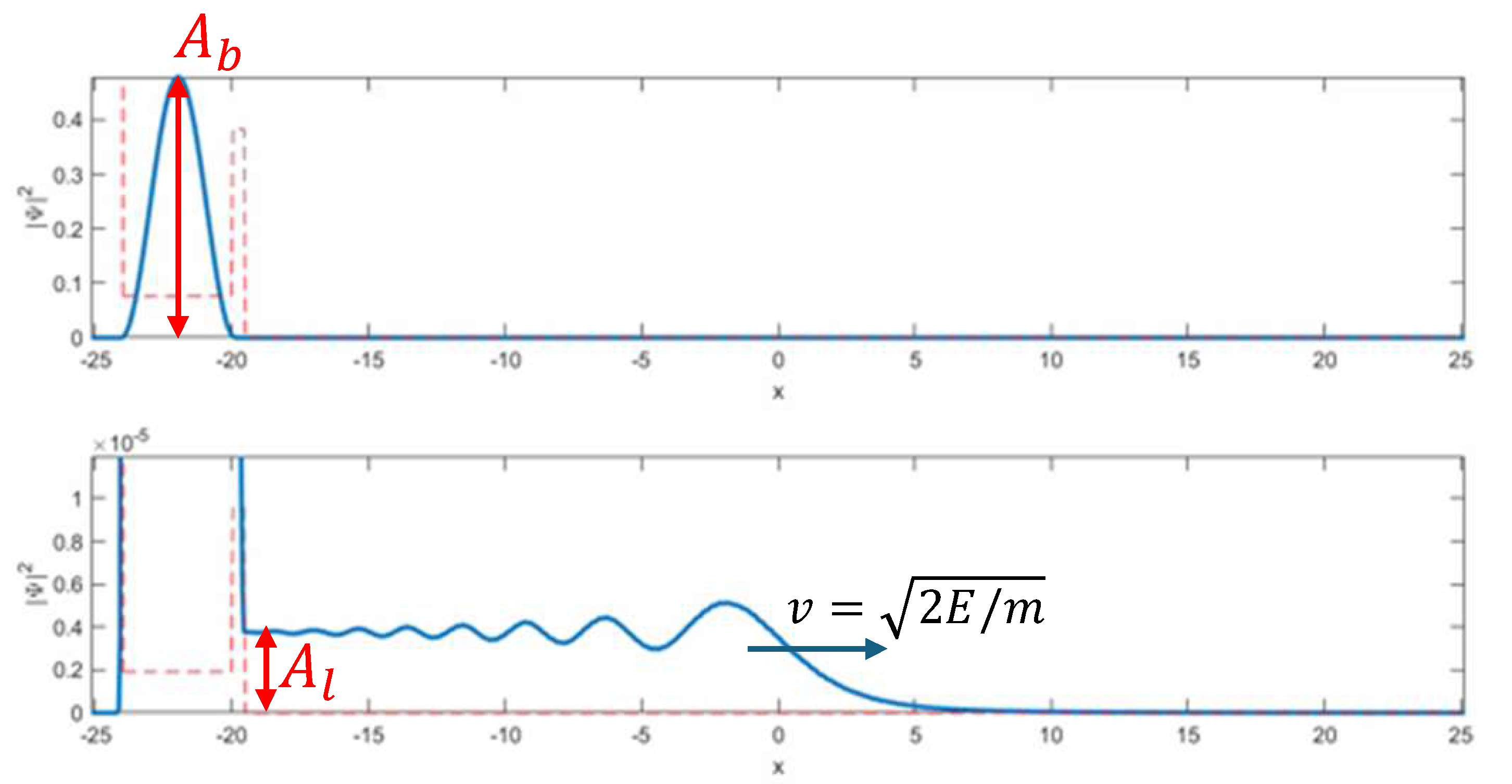
The important rate in this problem will be the rate at which the amplitude-squared of the wave function leaks out of the nucleus. This rate is given by the product of the amplitude squared \(A_l\) and the speed \(v\) at which the leaking wave function travels away from the nucleus. The speed is the group velocity \(v = \sqrt{2E/m}\), where the energy \(E\) will be set by the energy of the original bound state in the nucleus, including the offset of the potential due to Coulomb repulsion.
We will assume that the wave function is normalized so that at \(t=0\) we have \(A_b(0) \int f(x) dx = 1\). Defining \(\int f(x) dx = I\), the normalization yields \(A_b(0) = 1/I\).
As time progresses, the bound amplitude-squared \(A_b(t)I\) will decrease at the leakage rate, yielding the differential equation
\[I \frac{dA_b}{dt} = -A_l v.\]
Given the constant ratio between \(A_b\) and \(A_l\), we can substitute to obtain
\[\frac{dA_b}{dt} = -\alpha A_b v / I.\]
Solving the differential equation yields
\[A_b(t) = \frac{1}{I} e^{-\alpha v t/ I}.\]
From this, we already see that the integrated amplitude-squared still in the nucleus \(A_b(t) I = e^{-\alpha v t/ I}\), just like the probability of finding the nucleus not decayed after time \(t\) above, if we make the association \(\alpha v / I = \lambda\).
The amplitude of the red blobs will be set by the amount of amplitude transferred to the \(|e\rangle\) detector state in the time \(\Delta t\) between probe particles. We will assume that \(\Delta t\) is small enough that we can take \(A_l(t)\) to be constant over that interval. Hence we have the integrated amplitude squared (and hence probability) for the \(k^\mathrm{th}\) red blob
\[P_k = \eta A_l(k \Delta t) v \Delta t,\]
where \(0 < \eta \leq 1\) is the efficiency of the detector – the fraction of the amplitude-squared transferred from \(|g\rangle\) to \(|e\rangle\) by the interaction with the alpha particle.
Substituting \(A_b\) for \(A_l\), we obtain
\[P_k = \eta \exp{\left( -\frac{\alpha v}{I} k \Delta t \right)} \frac{\alpha v}{I} \Delta t.\]
Finally, if we identify \(\alpha v / I = \lambda\), then \(P_k\) is the same as expected from the conventional probability distribution above \(P(k \Delta t)\Delta t\), with the addition of the factor of \(\eta\). This makes sense, as the former expression was just about the probability that the nucleus decays, but the latter one is the probability that we successfully detect that decay. Note that the parameters that go into \(\lambda\) are set by the details of the confining potential of the nucleus. \(I\) is on the order of the width of the well, \(v\) depends strongly on the offset of the potential in the well, and \(\alpha\) depends strongly on the height and width of the barrier.
So our toy model reproduces the conventional result, but in a different way that suggests a very different picture. The conventional argument begins by assuming that there is a constant decay rate and calculating probabilities based on that. This includes an exponentially decreasing probability distribution of decay times, based on the result that as time passes it is more and more likely that the nucleus has already decayed. In contrast, in the model here there is a leakage rate, but it is not constant in time – it is exponentially decreasing. In this way, the exponential decrease is there from the beginning, and there is no instant when the nucleus decays. Instead, what we observe is just the imprint of the leaking alpha particle on a probe particle that interacted with the detector at a particular time.
It’s interesting to note that there seems to be some inherent timescales for the measurement of the decay, in contrast to the instantaneous jump posited in the conventional picture. First, there is the time it takes for the probe particle to interact with the detector. Second, there is the interval between probe particles. However, these time scales shouldn’t be interpreted as the time for a “quantum jump.” They are just the time it takes to get information about the state of the nucleus or alpha particle. If we can find a way to send in more probe particles, or have them interact faster, then we would measure the decay with higher time resolution. We would just produce smaller and smaller red blobs in greater numbers.
It is also worth pointing out the effect of the imperfect measurement of the alpha particle, and also the potential imperfect probing of the detector via the probe particles. It is not unreasonable that a single microscopic detector would probe decay of a single atom with less than perfect efficiency, as we have simulated above. When the leaking alpha particle wave function interacted with the detector, this led to a partial transfer of amplitude to the \(|e\rangle\) state, but also left a portion of the amplitude continuing on, correlated with \(|g\rangle\). This would correspond to a failure to detect the decay. Of course, in reality, there doesn’t have to be just one microscopic “detector.” As we will see shortly, there are typically a very large number of such detector particles. So even if the efficiency of each detector is low, it can become very likely that the alpha particle’s wave function will become nearly fully correlated with the \(|e\rangle\) state of some detector.
To keep things simple in the example above, we assumed that the probe particles had a maximal interaction with the detector. This is not necessary, however. We assumed above that the probe particle was completely transmitted after interacting with the detector in the \(|g\rangle\) state, and completely reflected after interacting with the \(|e\rangle\) state. This causes the red blobs in Fig. J.7 to completely split off from the green blob.
It is perhaps more realistic though that the two final states of the probe particle are not completely distinct (i.e. orthogonal). For example, the probe particle could be partially reflected and partially transmitted after interacting with the \(|e\rangle\) state. In this case, a portion of the red blobs would split off from the green blob in Fig. J.7, but a portion would remain overlapping with the green blob. Then, that remaining red blob would become more extended as the alpha particle continues to interact with the detector. When the next probe particle arrives, it is now a longer red blob that partially splits off and partially remains. The result is that the red blobs that split off in this case are more spatially extended in the \(x\) direction, and also overlap with each other in the \(x\) direction. This can be viewed as a reduction of the time resolution of the measurement – if we observe a particular red blob, the uncertainty in the alpha particle’s position spans the arrival of multiple probe particles.
Real quantum jump detectors
Now let’s compare the toy model above to two real implementations of devices for detecting quantum jumps. First, we will look at how Geiger counters can detect nuclear decay, and then how quantum jumps can be observed in the spontaneous emission of photons from an atom.
Geiger counter
A Geiger counter is a common device for measuring the presence of radioactive materials. It detects particles, such as alpha particles, emitted by radioactive decay.
The heart of the Geiger counter is a Geiger–Müller (G-M) tube, illustrated in Fig. J.9. The tube is filled with an inert gas. When an alpha particle travels through the tube, it can interact with an atom of the gas, ionizing it. This atom plays the role of a “detector” in the toy model. An electron originally bound to the atom is the state \(|g\rangle\), and the electron now traveling away from the ionized atom is the state \(|e\rangle\).
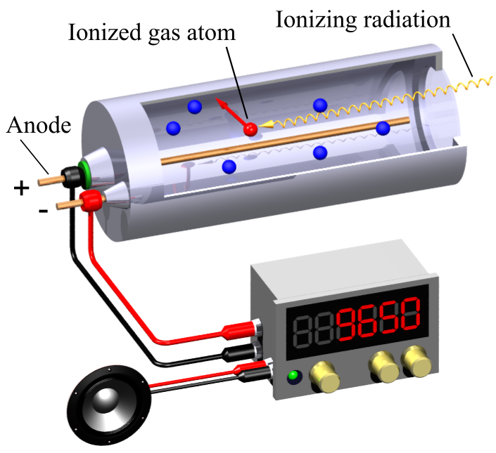
With the association of the \(|g\rangle\) state with a bound electron, and the \(|e\rangle\) state with an unbound electron, we can see why these two states will interact in significantly different ways with other particles in the environment. Moreover, a large voltage is applied between the a center conductor in the G-M tube and the outer wall of the G-M tube. This further distinguishes the \(|g\rangle\) state from the \(|e\rangle\) state, as the unbound electron is accelerated by this voltage.
In the G-M tube, the “probe particles” are other atoms that the unbound electron interacts with. The picture is slightly different than in the toy model, where the detector states both stayed localized at one position and were hit by incoming probe particles. Here both the electron in the \(|e\rangle\) state and the probe particles are moving. But the idea is the same: now an unbound, accelerated electron in the \(|e\rangle\) state can interact with another atom in the gas, causing that atom to become ionized. So if the “detector” atom remains in the \(|g\rangle\) state, an electron in the “probe particle” atom remains in its original, bound state. But if the “detector” atom is in the \(|e\rangle\) state, that electron in the “probe particle” atom is in a very different unbound state.
Note that just as the nucleus does not decay by a sudden jump in this picture, the atoms are not ionized by a sudden jump either. Instead, the amplitude is continuously transferred from the bound electron state to the unbound electron state, though this process is much faster than the nuclear decay we have been considering.
This now takes us as far as the simulations above have shown. The alpha particle wave function is leaking into the G-M tube. As it begins to interact with an atom in the tube, amplitude begins to be transferred from the bound electron state to the unbound electron state. Once the expanding wave function of the unbound wave function component interacts with another atom in the gas, ionizing it, we now have the entangled state represented by the splitting off of a red blob in Fig. J.7. The leaking alpha particle wave function continues to interact with the detector atom, transferring more amplitude to the \(|e\rangle\) state. When this interacts with another atom in the gas, another red blob splits off along another dimension.
As discussed above, the splitting off of the red blobs is the first step in decoherence and/or measurement. We can carry the process forward and see how we end up performing a measurement with the G-M tube. For a human to perceive the outcome, the effect of the alpha particle interacting with an atom must be amplified up to a macroscopic scale. This can be accomplished via a chain reaction, where the initial microscopic interaction sets off an avalanche, essentially propagating the information to many particles.
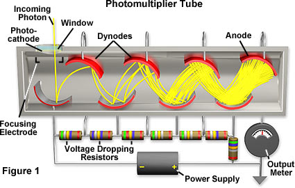
The chain reaction in the G-M tube is the Townsend avalanche, depicted in Fig. J.10. We have already seen that the electron released by ionization of an atom by the alpha particle is in turn accelerated and ionizes another atom, releasing another electron. It may not be surprising then that next both the original electron and this newly unbound electron get accelerated, and can ionize more atoms. Eventually, we get a large enough number of unbound electrons so that when they arrive at the central conductor in the tube, the flow of electrons is measurable as a current pulse. Hook this current up to a speaker, and we get an audible click!
The Townsend avalanche in Fig. J.10 is directly analogous to the avalanche of electrons produced in a photomultiplier tube, as discussed in the section Amplification and decoherence. Likewise, a similar chain reaction is described in the “marble run” measurement device there. Note that still, the evolution of the wave function does not describe a single avalanche. Instead, it describes a separate avalanche correlated with each red blob. Each ionization of a probe particle at a different time results in an avalanche in that part of the wave function. Due to the large number of particles involved, the part of the wave function correlated with each avalanche becomes very well separated in the high dimensional configuration space, and thus produces clicks at different times in different “worlds.”
Spontaneous emission
Spontaneous emission of a photon from an atom is a process similar to the nuclear decay considered here. In that case, an electron bound to an atom is initially in a high energy state. The conventional picture says that there is some constant rate for the electron to spontaneously jump to a lower energy, emitting a photon. This leads to exactly the same probabilities as for the case of nuclear decay, such as a constant probability of emission in any time interval (assuming emission has not yet occurred), and an exponentially decreasing probability distribution for the emission time.
Here, however, we’ll present a picture where jumps only appear to occur due to interactions with the environment. This discussion will be a little hand-wavy because the case of photons is not represented by the Schrödinger equation simulations above, which only works for massive, non-relativistic particles. But the ideas should work out the same.
Like nuclear decay, spontaneous emission can occur over a large range of timescales, ranging perhaps from picoseconds to hours. The longer end of the range makes the “quantum jumps” particularly noticeable – it can be possible to monitor the system fast enough to observe the jumps. This was first demonstrated experimentally in 1986, in papers from two groups, led by Hans Dehmelt and Dave Wineland (PRL 56 (26) 1986, and PRL 57 (14), 1986). The Dehmelt paper makes the comment, “These experiments have a special fascination, as, in the language of modern quantum mechanics, they allow one to watch the reduction of the wave function by the measurement process on the oscilloscope screen.” Here, of course, we will attempt to explain these results without any “reduction” of the wave function.
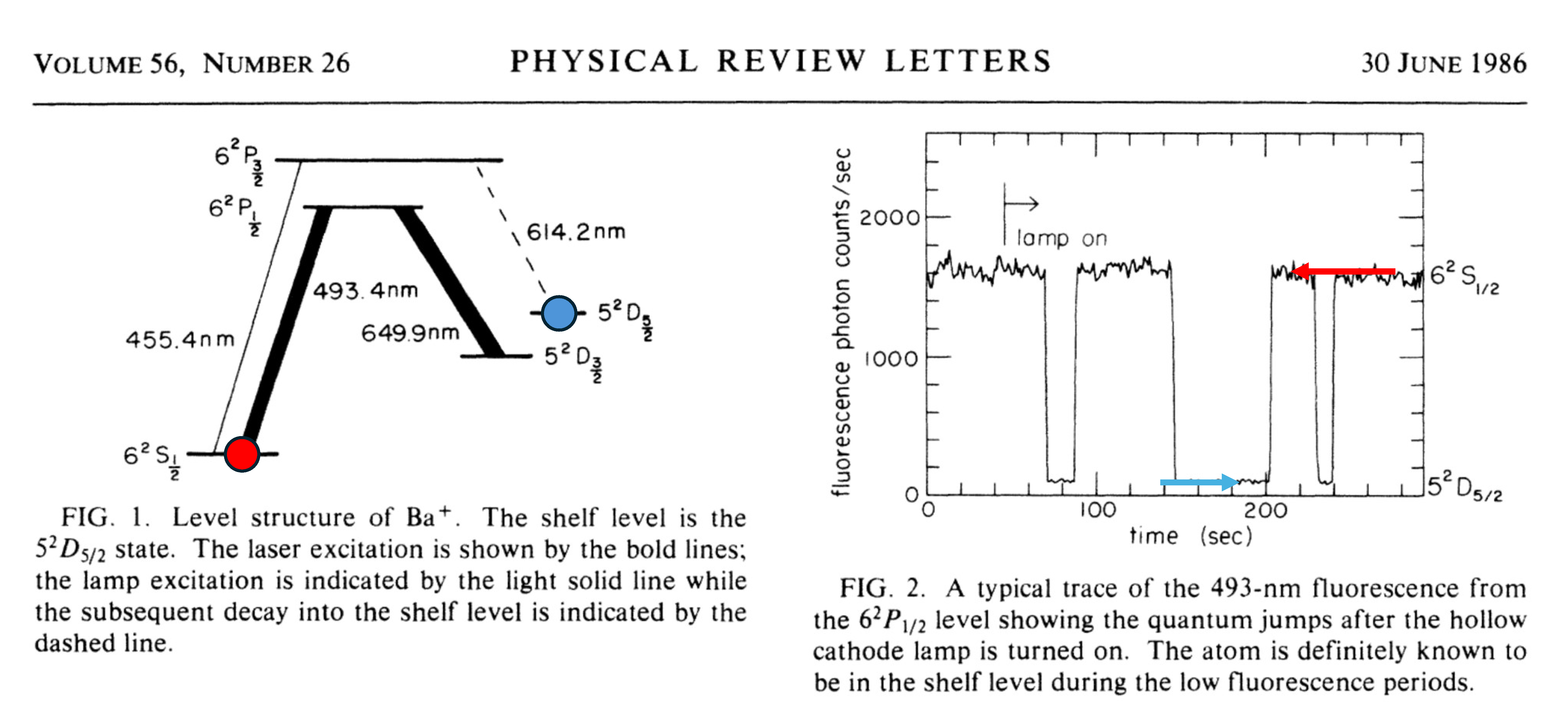
The scheme and main result from the Dehmelt paper is shown in Fig. J.11. The system undergoing the “jumps” is a single Barium ion, trapped and laser-cooled in ultra-high vacuum. This is the same technology that led to today’s ion trap quantum computers.
The horizontal lines in the diagram at the left of Fig. J.11 show the energy of several different states for an electron bound to the Barium ion. The lines connecting the states indicate how strongly light can be emitted or absorbed between these states, at the labelled wavelengths. Without going into all the details, we can consider an electron bound to the atom initially in the state marked by the blue dot. Note that there is no line connecting that state to a lower-energy state. This is because the transition from that state down to the state marked with a red dot is so weak that they didn’t even put a line there – its spontaneous emission time is around 30 seconds. This is the quantum jump we will be looking for.
In principle, we could watch for the jump by trying to detect the photon emitted when the state jumps from the blue dot to the red dot. The problem is that it is hard to detect individual photons with high efficiency, so if the atom is only emitting one photon every minute or so, it’s just not going to work. Besides, we will see that the scheme used here permits us to monitor the state as the process plays out.
The key to the scheme is that a laser is incident on the ion at a wavelength of 493 nm. Because the ground state (with the red dot) is connected to another state via this wavelength, these photons from this laser will scatter strongly from the ion if the electron is in the ground state. If the electron is in the state marked with the blue dot, the photons cannot scatter.
The result is that when the electron is in the blue dot state, no scattered photons are observed. But when the electron jumps down to the red dot state, we see lots of photons scattered. The data at the right of Fig. J.11 shows this playing out. When the photon count rate is low, we know that the electron is in the blue dot state. Then at some point we see the photon count rate jump up – apparently the electron has suddenly jumped to the red dot state!
So to apply the toy model here, the electron starts in the blue dot state. Amplitude from the blue dot state slowly and gradually starts to leak to the red dot state which is correlated with the emission of a photon. This is like the nucleus gradually changing from U-238 to Th-236 as the alpha particle slowly leaks from the nucleus.
In this case, instead of interacting with the emitted particle, the probe particles will interact with the ion itself. Here, the probe particles are the 493 nm photons. They do just what we want: when the electron in the ion is in the initial blue dot state they do not interact, but if the electron is in the red dot state, they interact strongly, likely scattered off in a new direction. For the sake of simplicity, we will assume that the photon will be scattered in this case with perfect efficiency.
So the process plays out as follows. The amplitude starts slowly transferring from blue to red. When the first probe photon arrives, an entangled state results. The two components of this entangled state correspond to electron in the blue state with the photon passing by, and the electron in the red state with the photon scattered. The latter component corresponds to the splitting off of a red blob in Fig. J.7. The first component of the state corresponds to “no jump yet”, and the second component corresponds to “immediate jump.”
After the first probe photon has split off the red state amplitude, more amplitude is transferred from blue to red, correlated with the case of no photons yet scattered. Now the second probe photon arrives. It, too, will split off a new red blob, now correlated with “first photon not scattered, second photon scattered.” The second probe photon also interacts with the red state component correlated with the first probe photon scattering – the second photon will also be scattered, so this red blob is now correlated with “both probe photons scattered.”
The language in the preceding paragraph was getting a little hard to follow. So let’s refer back to Fig. J.6. There we introduced notation that will allow us to keep track of which probe particle was not scattered (\(|0\rangle\)) or scattered (\(|1\rangle\)). With three probe particles, we could have a state such as \(|011\rangle\), meaning 1st and 2nd photons scattered, 3rd not scattered.
Following the example of Fig. J.6 we see successive entangled components emerging as each probe photon arrives. These components are correlated with the red state, meaning the electron has jumped down. Each entangled component is also correlated with some state of the probe photons that looks something like \(|111...111000...000\rangle\). That is, some number of ones (at least one) followed by some number of zeros. As before, each 0 or 1 indicates which probe photon was scattered or not, with the earliest probe photon at the right.
These states of the probe photons correspond to “no photons scattered for a while, then all photons scattered after some point.” Note that this is precisely what we see in the data at the right of Fig. J.11, for example, from the blue arrow to the red arrow.
So we see that the data in Fig. J.11 correspond to one particular red blob. (At least the portion of the data between the blue and red arrows; there is an additional light source in the experiment that resets the electron to the metastable state effectively repeating the experiment multiple times.) A different red blob would show a jump at a different time.
As we know, we are going to associate each red blob with a different “world.” So far, the blobs are different components of an entangled state with spatially separated photon positions, but we have not yet seen the massive entanglement needed to be sure that they will evolve as separate worlds. This will occur when the information about the jump undergoes amplification and decoherence, i.e. measurement.
To amplify individual photons scattered from a single ion, Dehmelt and Wineland both use a photomultiplier, already introduced in the section Amplification and decoherence. The diagram of a photomultiplier shown there is reproduced here in Fig. J.12.
The first step in detecting a photon with a photomultiplier is when the photon interacts with a material called the photocathode. This is a material whose electrons are particularly weakly bound, so that the incoming probe photon can kick out an electron via the photoelectric effect. Once a probe photon has performed this ejection of an electron, the blobs of the wave function with that photon scattered are now separated from those without that photon scatterd along additional dimension(s) – that corresponding to the position of the ejected electron.
Next comes the chain reaction that amplifies the information, and also separates the different blobs of the wave function in a vast number of dimensions. The electron ejected from the photocathode is now accelerated by a voltage, and hits a piece of metal. That electron now has enough energy to knock several electrons out that metal. These electrons in turn are accelerated and each knock several more electrons out of another piece of metal. This process continues until there are enough electrons to be measurable as a current in a circuit. Note that this is very similar to the Geiger–Müller tube, where the cascade involves knocking electrons loose from atoms in a gas instead of a solid metal.
Each time more electrons are knocked loose from the metal, the blobs of the wave function are separated along more dimensions. The cascade only takes place in components of the wave function where a given probe photon has been scattered (and hence the electron is found to have jumped to the ground state at the time of that probe photon’s arrival).
By the time the amplification is finished, even two blobs that only differ by a single probe photon scattering are now separated over a macroscopic number of dimensions. That is, we can now consider these to be two separate worlds that differ only by the “quantum jump” occurring at times separated by the arrival of two successive probe photons. Again, this is assuming that the photons are perfectly scattered by the ion in the ground state, and we can collect and measure them with perfect efficiency. If not, then our time resolution will be decreased accordingly.
In the end, the implication is that there are now many distinct components of the wave function, each corresponding to a different time for the quantum jump. Each gives a different version of the plot shown in Fig. J.11. Each well-separated blob in the wave function is correlated with a different pattern of electrical pulses in the photomultiplier. These different patterns get translated into different photons emitted from the oscilloscope screen in Dehmelt’s lab. Now correlated with each blob, there are different components of the wave function of the particles making up the body of a researcher in Dehmelt’s group, observing different patterns on the oscilloscope. We can continue tracing the non-interfering paths of the different blobs. Different versions of PRL going to press. Different versions of me cutting and pasting from a pdf of that PRL 40 years later. Different versions of you seeing that plot on the Catland website.
Perhaps we can close this section with the question, “Wait, but do these worlds actually exist?” I do not know the answer to this question. I am not even sure what it means for something to “exist.” What I aim to show here is that the wave function as given by the Schrödinger equation can be understood in this many worlds picture, and that this picture is consistent with what we observe.
Whence wave packets
As a coda to this section, let’s discuss wave packets. Throughout Catland, examples have been based on wave functions in the form of localized wave packets. This is certainly handy for visualization, as it makes a particle look sort of like our classical notion of a particle: mostly localized in position with a fairly well defined momentum. But is this at all realistic? How often in the real world do particles actually have such a wave function?
I will argue that viewing free particles as wave packets may not be so far from the typical reality, though with maybe some extra complications.
In the model of nuclear decay above, we start with a wave function for the alpha particle that does not look like a free well-localized wave packet. The unbound part of the wave function just spreads out to a very large scale over time. However, the interaction with the localized detector, and then the localized probe particles renders well-separated components in which the alpha particle wave function is a localized wave packet. Note that its not that the delocalized alpha particle wave function is somehow being squeezed into a wave packet, but that bits of it are becoming correlated with other localized parts of the wave function.
So we see that an interaction that depends on position can essentially cause an extended wave function to split into well-separated localized wave packets, if it interacts with something spatially localized.
The same result has been obtained in a more mathematically sophisticated way, by looking at the decoherence of a 1D free particle interacting with a bath of harmonic oscillators (see Zurek, Rev. Mod. Phys. 75, 715, 2003). Here, the interaction depends on the distance to the harmonic oscillator. The result is that the 1D particle decoheres into Gaussian wave packets, whose width depends on the strength of the interactions.
In the examples above, the different worlds wind up being distinct blobs within the wave function, well-separated along many dimensions. However, it may also be possible to have the same type of behavior, but in a continuous case instead of the discrete case.
Figure J.13 illustrates a simple example of continuously separated parts of a wave function. The initial state is shown on the left. Here, particle A is in a wide packet, and particle B is in a narrow packet. Particle A has much greater mass than particle B, and initially, particle B is moving towards the stationary particle A. As such, the wide blob will move vertically downwards. If the particles strongly repel at short distance, then the wave function will reflect when it hits the white diagonal line. The rightward edge of the blob will collide first. Since particle A is much heavier, it will barely recoil, sending the blob straight back up. The result is that, after completely reflecting, the blob becomes stretched out to become diagonal as it heads vertically upwards.
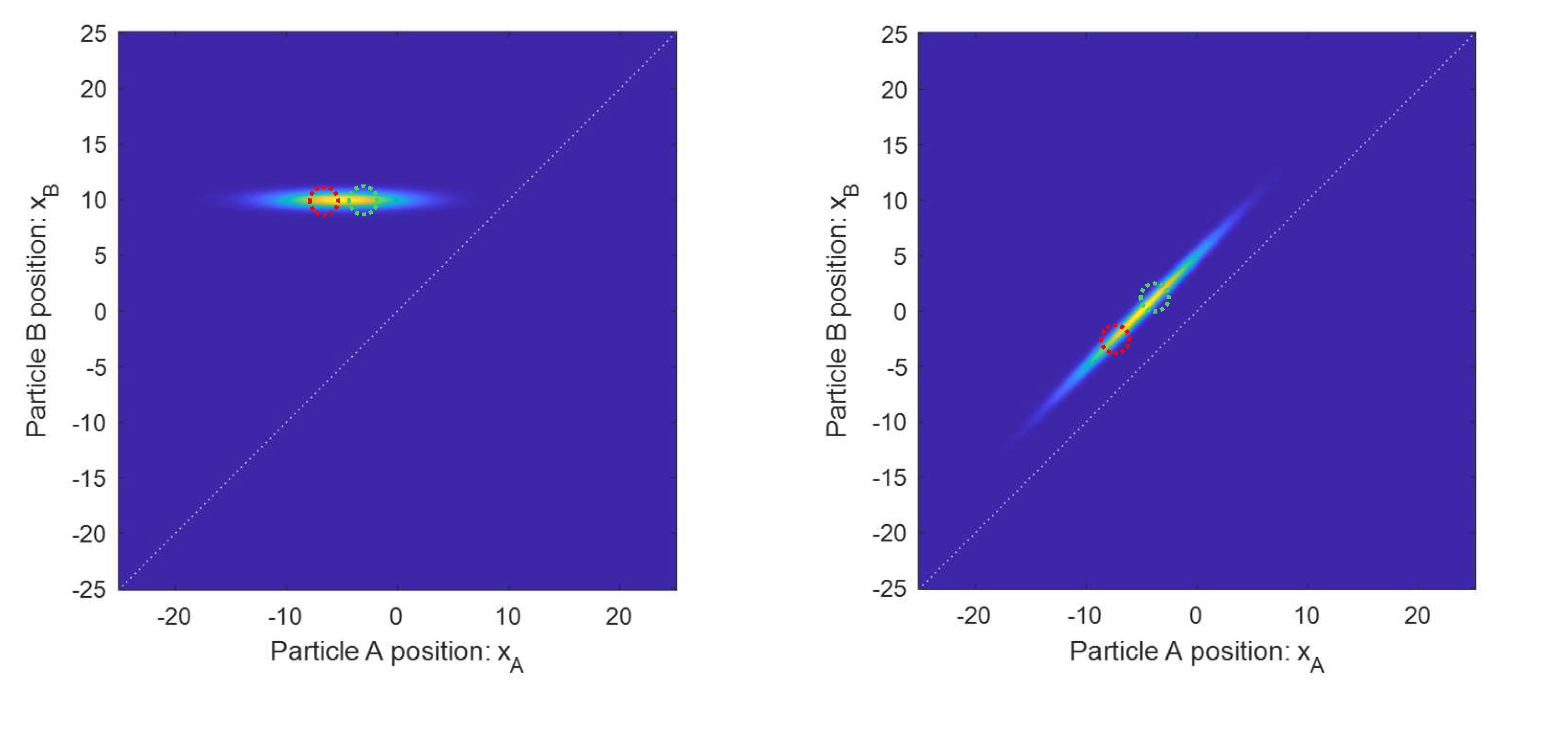
The end state in Fig. J.13 is still a single blob, but the different parts of the blob are misaligned from each other. This is highlighted by the red and green dotted circles. These are at the same \(x_A\) positions in both panels. They start out aligned along the horizontal direction, but end up misaligned.
If the two dotted circles represented the positions of two blobs, we might consider them to be on the way to becoming separate worlds. Instead, we might imagine that this wave function goes on to collide with more particles, which could tilt this long diagonal wave function in more dimensions. The red and green dotted circles could then become misaligned in many dimensions, despite being connected by nonzero amplitude in the wave function.
The stretched out wave function in many dimensions yields a picture where different regions of the wave function can be considered to be well-separated, as long as they are sufficiently far apart so as to not be aligned along any axis. Indeed, this is the picture that results from the calculation of a particle interacting with a bath of harmonic oscillators. An initially delocalized particle decoheres into a continuum of localized packets, entangled with different states of the oscillators.
So we see that the toy model above presents a simplified picture of how quantum jumps occur. An actual many-particle wave function is probably much more complicated than the simple blobs moving around. It is at least plausible however that the blobs depicted above yield the correct intuition with which to understand the more complicated realistic behavior of an \(N\)-dimensional wave function.